As an appendix promised for the article How fast helium balloon floats…, and also appendix for the follow up article Hint for solving quadratic drag force on a damping oscillator, I’m going to show the phase plot or phase diagram of the oscillation of quadratically damped floating balloon.

Originally, I want to make it interactive, but I realized the computation is complicated, it might make your browser hangs. I am using GeoGebra instead to make some screenshots of it.

Recalling the equation of motions

Our original equation of motions is this:

$\ddot x=-\omega^2 x - d \dot x \left| \dot x \right|$

In the previous article we call $d$ as $D_2$ the damping coefficient for quadratic drag force. Because we are very clear now that this article only consider quadratic case, let’s just call the coefficient $d$.

The equation of motion above have interesting property. It will converge to a stable position, $x=0$ and $\dot x=0$ and $\ddot x=0$, due to losing energy. That means, the center of the coordinate system is the position where the object converges and stop moving.

Any oscillation with linear restoring force $-\omega x$ and quadratic damping drag force $- d \dot x \left| \dot x \right|$, can be reduced into a generic equation above. If the equation have constant force $C$, we shall find $C=\omega A$ where A is the amplitude value that can be used to do a coordinate shift from the original reference frame to a reference frame where position 0 is where the object will be at rest.

So, it’s suffice for us to find the behaviour of above equation, because any similar motions can be reduced to our equation above.

The term in the drag force $- d \dot x \left| \dot x \right|$, the absolute value of $\dot x$, is just a convenient way for us to say that the direction of the drag force is always opposing the direction of the velocity. With the magnitude of drag force proportional to $\dot x^2$.

So, our equation above can be broken down into positive (positive x) direction and negative (negative x) direction.

$\dot x >0; \ddot x=-\omega^2 x - d \dot x^2 \\ \dot x <0; \ddot x=-\omega^2 x + d \dot x^2$

We solved the phase space equation in the previous article. We also defined more variables that will make our life simpler.

$X=2dx \\ V^2=\frac{2d^2}{\omega^2}\dot{x}^2 \\ \alpha =\frac{2d}{\omega^2}\ddot{x} \\ K_+=\frac{k_+}{\omega^2} \\ K_-=\frac{k_-}{\omega^2}$

The phase space relations conveniently becomes:

$V > 0; K_+=e^X(1+\alpha) \\ V < 0; K_-=e^{-X}(1-\alpha) \\ V > 0; K_+=e^X(1-X-V^2) \\ V < 0; K_-=e^{-X}(1+X-V^2)$

Some interesting insight from this. When we normalized the phase space variables $X$ and $V$, it seems that the phase is deterministic. The constant $K_+$ and $K_-$ is entirely defined by the substitution of $X$ and $\alpha$. That means, for any such system with this behavior, we can transform the initial condition to fit such phase plot. Then find the solution and behavior, then transform back from this standard plot.

Now, let’s define our standard initial condition.

First, we define that our standard coordinate system $x=0$ is a position when the motion has converges.

Second, we define that our initial condition start when the object is displaced from $x=0$, with maximum displacement. We can pick either in the left side or right side of origin. But I prefer to start from the left side. By starting from the left side, we will use the positive equation of motion (where velocity direction is positive).

If the distance between initial position and $x=0$ is $A$ (the maximum amplitude). Then the initial position $x_0=-A$. The initial acceleration becomes the maximum acceleration possible, and we can easily calculate it using Newton’s First Law in the initial condition. Or, shortly $a_0=\omega^2 A$

After defining the initial condition above, we have completely mapped a phase from our standard phase space $X$ and $V$ into the actual phase space of the object $x$ and $\dot x$.

Drawing the plot of first iteration

To illustrate, we are going to do a transformation $X=2dx$. this will map $x_0=-A$ into $X_0=-2dA$. From the initial condition, we got the constant $K_+$

$K_+=(1-X_0)e^{X_0}$

The constant for our standard phase is determined by it’s original position.

If we use Lambert W function to find $X$ at $V=0$, we should find two values of $X$. One at $X_0$ when the object began to move and another one at $X_1$, which is when the object stop and change it’s velocity direction.

$X=1+W(-\frac{K_+}{e})$

By the way, we got the above expression using Lambert W substitution: $w e^w = z$ into $w=W(z)$, with $w=X-1$.

Most of numerical $W$ function only implements the principal branch. But the equation above has two solution, which means it will use two branch of $W$ function, the principal and $W_{-1}$ branch. Luckily for us, the $W$ function returns the other $X$ value, $X_1$ and not $X_0$ again. This is probably because the absolute value of $X_0$ has to be bigger than $X_1$ due to the damping.

With just this information we are able to plot the phase. The equation is:

$V=\sqrt{1-X-K_+e^{-X}}$

It looks like this (plotted using GeoGebra):

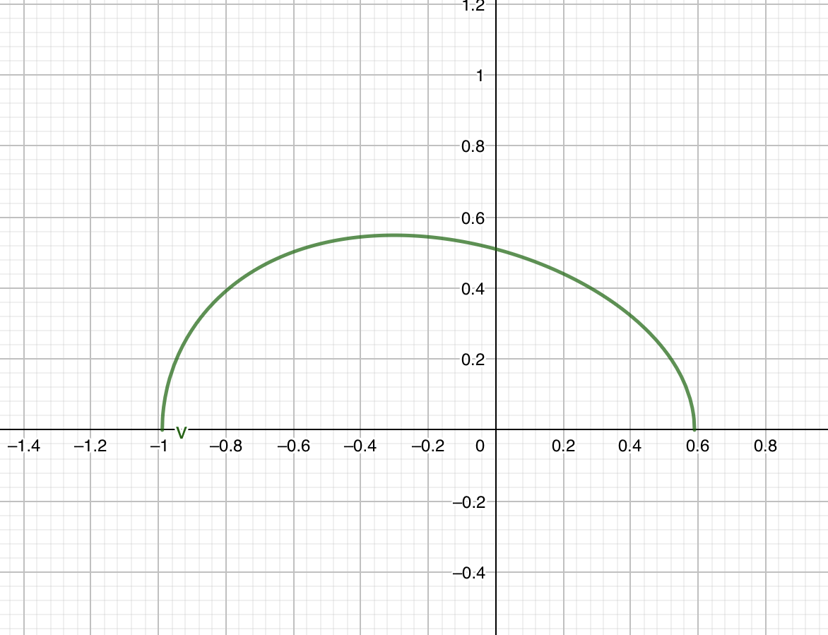
As you can see that the maximum of $V$ is slanted a little bit left. We can calculate this position using the acceleration relation above, setting $\alpha=0$.

$X_{peak}=\ln(K_+)$

Drawing the plot of the second iteration

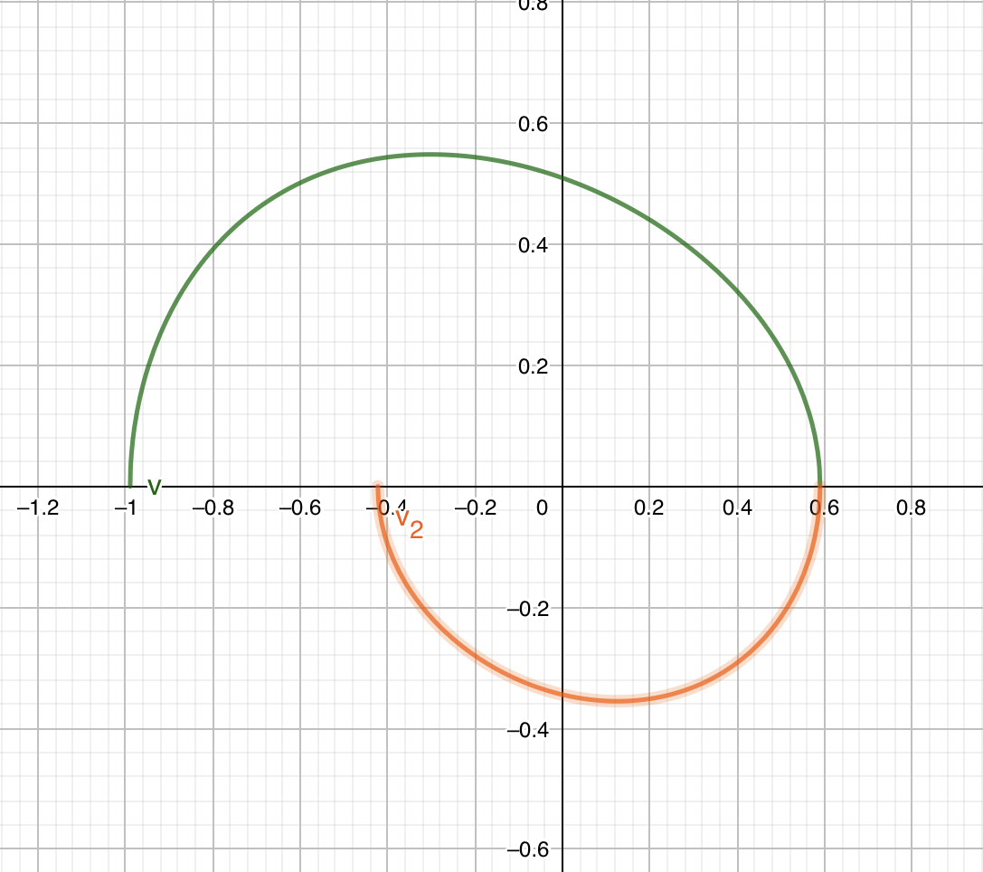
The second iteration of the phase is when the velocity is in the negative direction. So, we use the second set of the equation:

$V=-\sqrt{1+X-K_-e^{X}}$

The initial $X$ value is the value that we find before: $X_1$. From there, we calculate $K_-$

$K_-=(1+X_1)e^{-X_1}$

Then, we can calculate $X_2$.

$X=-1-W(\frac{K_-}{e})$

The peak:

$X_{peak}=-\ln({K_-})$

The plot looks like this:

The plot for the next n iteration

By this point, you probably have found some patterns.

Our equation basically tells us the same shape of phase, but it is rotated, and scaled, due to the Lambert W function behaviour.

Let’s do a small recap. Our most basic relation tells us this:

$V^2=1-X-Ke^{-X}$

It will have two zeroes, $X_0$ will be negative and it’s absolute value is bigger than the positive $X_1$

The peak is only determined by $K$, which is $X=\ln(K)$.

$K$ is determined only by it’s initial position.

$K=(1-X_0) e^{X_0}$

Or the other way around is also valid. It’s starting initial position is determined by $K$.

The equation when $V$ is negative is actually the same equation but with a transform $X'=-X$ and $K'$. After that, the equation just alternates it’s sign with different value of $K$.

We can reformulate which equation/constants to use based on which iteration number.

Note, that if we define $K_0=0$, there is only one $X$ value possible, which is 1. We can imagine that the original amplitude $X_0$ is so far away at $-\infty$ that it technically doesn’t cross $X$ axis. Let’s use this as a base.

$X_0=-\infty \\ K_0=0 \\ X_1=1$

We got the next $K$, $K_1$ by flipping the equation, so the amplitude now is $X=-X_1=-1$. I’m sure you got the pattern if you continue through multiple iteration. We got this relation:

$X_n=(-1)^{n-1}(1+W(\frac{K_{n-1}}{e}) \\ K_n=(1+(-1)^{n-1} X_n)e^{(-1^{n-1}) X_n} \\ V_n=(-1)^n \sqrt{1+(-1)^{n-1} X- K_n e^{(-1^{n-1}) X}} \\ X_{peak-n}=(-1)^n\ln(K_n)$

Choice of index $n$ is completely arbitrary. With this kind of choice, that means, when $n$ is even, velocity is positive. When $n$ is odd, velocity is negative.

From this recursive relation, you can make a simple program that calculate all the necessary points of interests.

It’s also worth noting that subsequent values of $K_n$ is only determined by the initial values in the range of $-\infty < X_0 \leq -1$. If $X_0$ were to happen in the range $-1 < X_0 < 0$ it is probably not the first iteration, and you can determine the the original $X$ that is capable of generating that value.

Simply speaking, if you make a phase plot with $X_0=-1$ then you will get the same phase plot if you draw the same plot, but starting at $X_2$ that is generated from $X_0=-1$. So, hypothetically speaking, if we have a canonical phase plot and the other phase plot can be transformed into this canonical phase plot, that means it is possible to define a standard function that will cover the whole dynamics.

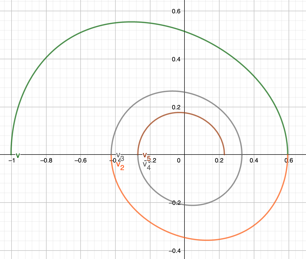
Other insights from the above recursive relations is the maxima/minima of each cycle, from the value of $X_{peak-n}$. We can infer that eventually $K_n$ will converge to 1. In which the $X_{peak-n}$ will converge to 0.

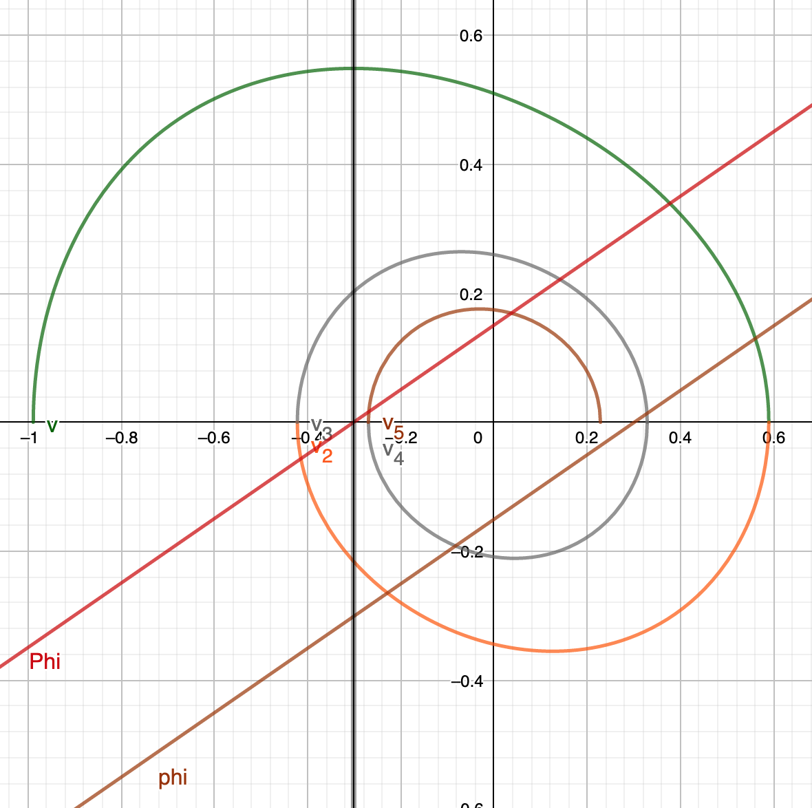
This is a plot of graph with $X_0=-1$ with 5 iterations:

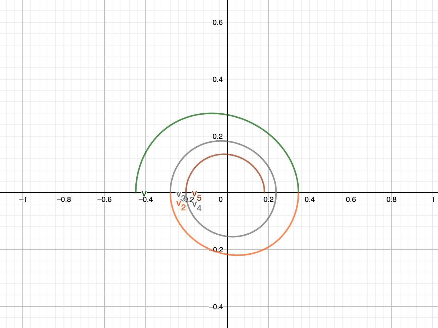
Same plot with but now with $X'_0=X_2$, also with 5 iterations as you can see, same plot is constructed:

Deriving interesting identities

We can go a little bit further deep. There is an interesting relation that we don’t have if the plot phase is a simple harmonic cycles. If we choose two arbitrary index of a different parity $K$, with the same value of $V^2$. We have an interesting relationship between positive $V$ and negative $V$. Obviously in the different half cycle, it will corresponds with a different $X$ value that maps to the same $V^2$. With simple harmonics, this is not interesting because the $X$ value will be the same, but with this plot phase, we will have extra identity. Let’s suppose that $X_a$ is the position where velocity is positive, meanwhile $X_b$ is the position where velocity is negative.

$1-X_a-K_ae^{-X_a}=1+X_b-K_be^{X_b} \\ K_be^X_b-K_ae^-X_a=X_b+X_a \\ H \sinh(\phi)=\frac{X_b+X_a}{2}$

We just introduced a new variable $H$ and hyperbolic angle $\phi$. For every same $V^2$ between consecutive half cycles, this relation emerges. The definition of the new variables:

$H=\sqrt{K_a K_b}e^\frac{X_b-X_a}{2} \\ \phi=\ln(\sqrt{\frac{K_b}{K_a}})+\frac{X_b+X_a}{2}$

We can do lots of things with this relation. For example, one of the things I immediately recognize is the term $\frac{X_b+X_a}{2}$ shows up twice in the identity above and the definition of $\phi$. That means we can use the identity to approximate something using recursion.

We know that in the final iteration, the value of $K=1$, because the peak has to be in the middle. We can then inspect every $X$ where $V^2=0$. By setting either $K_a$ or $K_b$ to 1, then, $H$ quantifies how far the current cycle is with the final cycles. This is set unambigously because either Odd $X_a$ or even $X_b$ will corresponds to a positive value of $X_b-X_a$. For example if $X=1$ then it must be $X_b$ due to the recursion definition above. If $X=-0.59$ then it must be $X_a$, causing $X_b-X_a=0.59$.

If we compare with $X_0$, then $H\approx \infty$ which is the maximum value. When $X=1$, $H=\sqrt{2}$. We can immediately know which cycle is earlier or later. We can even compare different $H$ to get relative cycle between the two. The idea is very powerful, that we can think about $H$ as the absolute cycle lengths. Then $H_a$ and $H_b$ can be divided to get a relative cycles. We can even know, if $\sqrt{2} < H$ then that means it is the very first initial cycle.

Now, we are going to try to interpret the hyperbolic angle $\phi$. We can immediately recognize that it is possible to set the right hand side to zero. But the cycle length $H$ can not be zero. So the zero must comes from $\sinh(\phi)$. The reason why it happens, maybe because of these:

First, $X_a=-X_b$ whatever that is. But in order for that to be valid. It also must satisfy

$\ln(\sqrt{\frac{K_b}{K_a}})+\frac{X_b+X_a}{2}=0 \\ K_b=K_a$

Because we assumed that $K_b$ and $K_a$ from a different parity of $n$, that means this can only happen if $K=1$ and it is in the final cycle. We actually proved otherwise. The $\phi$ then cannot be zero if we are inspecting two cycles from a different parity.

If we define, the absolute cycle length of cycle n as $H_n$:

$H_n=K_ne^x$

Then our previous $H$ is actually a square root/geometric average between two absolute cycles:

$H=H_{average}=\sqrt{H_a \cdot H_b}$

While $\phi$ can be defined as half the difference between two absolute cycles, and can be interpreted as hyperbolic angle difference:

$\phi_n=\frac{1}{2}\ln(H_n)=arctanh(\frac{H_n-1}{H_n+1}) \\ \phi=\Delta \phi=\phi_b-\phi_a=\frac{1}{2}\ln(\frac{H_b}{H_a})$

The quantity $\phi$ can becomes a natural choice to understand which cycle is currently early or late if we compare them. We can retrieve the cycle’s hyperbolic angle from any absolute cycle length $H_n$, either by calculating it directly with the natural logarithm, or by using $arctanh$ Like what we understand before. But now, we can conveniently give it a name. It arises intuitively that when $\phi$ is small, that means the cycles is at it’s end and very similar.

From these results and understanding, we can then try to generalize these identities.

It follows that it turns out this identity is valid for any time that we observe two different cycles with the same $V^2$.

$H_{avg} sinh(\Delta \phi)=X_{avg}$

However, remember that the sign alternates whenever if it’s not the same parity. Currently, the above identity holds if $b$ odd and $a$ even.

It is a direct result, that if we compare two different $X$ in the same even cycle (positive velocity) with $X_b > X_a$:

$K_+ e^\frac{{-X_b-X_a}}{2} sinh(\frac{X_b-X_a}{2})=\frac{X_b-X_a}{2}$

In the odd cycle (negative velocity)

$K_- e^\frac{{X_b+X_a}}{2} sinh(\frac{X_b-X_a}{2})=\frac{X_b-X_a}{2}$

From both equation, we can’t determine if we set $X_a=X_b$, which is make sense because the only time it happens is when $X=X_{peak-n}$.

If both $X$ are zeroes of the equation, then $\left|X_b-X_a\right|$ is the full range/length of $X$ of that cycle. We can call this the span $S=\left|X_b-X_a\right|$. Meanwhile the quantity $\frac{{-X_b-X_a}}{2}$ and $\frac{{X_b+X_a}}{2}$ turns out to be always positive due to the slanted shape of the phase plot. It is the average of absolute value of left and right amplitude difference. Let’s call this $\Delta A$.

$K e^{\frac{\Delta A}{2}} sinh(\frac{S}{2})=\frac{S}{2}$

Regardless of if it is an odd or even cycle, $\Delta A$ is actually a good quantity to compare against difference cycles. If $\Delta A$ is small or near zero, that means it is closer to final cycle. If we remember our definition of absolute cycle length $H_n$. Then the value $K e^{\frac{\Delta A}{2}}$ is a relative cycle length between the same span of cycle $H_{avg}$.

With this property, we can easily scale any phase plot with a given span $S$ into another span. If we treat span as a continous variables (we don’t have any reason now, but for the sake of arguments, let’s pretend), we can take partial derivative. A span is invariant under origin translation. That means, in any given cycle, if we know the span and the motion constant $K$, we can determine where the canonical origin should be from the $\Delta A$ value.

Next, we are going to observe the quantity $\phi$.

The $\phi_n$ is an equivalent of $H_n$ but it is in the form of hyperbolic angle. Since we have :

$\phi_n(X) = \frac{1}{2}\ln(H_n(X))$

It’s value may signify some importance with the hyperbolic geometry. The range of values of $\phi_n(X)$, depends on it’s span and amplitude difference in a given cycle $n$. The minimum value $\phi_{n,min}=-\frac{S+\Delta A}{4}+\frac{1}{2}\ln(K_n)$, the maximum value $\phi_{n,max}=\frac{S-\Delta A}{4}+\frac{1}{2}\ln(K_n)$. It’s very similar with the phase of circular function like, $\sin(\theta)$. I’m very suspicious. The midpoint of $\phi_n$ is a very special value where $\phi_{n,mid}=X_{peak-n}=\ln(K_n)$.

From, that we have an interesting hyperbolic identity, where any hyperbolic angle $\phi_n(X)$ can be described with relative to the midpoint. Then, we have a quantity to for us to actually which phase the oscillation is currently in with arbitrary $X$ value.

$\Phi_n(X) = \phi_n-\phi_{mid}=\frac{1}{2}\ln(\frac{e^X}{K_n}) \\ \Phi_{n,min}=-\frac{S+\Delta A}{4}-\frac{1}{2}\ln(K_n) \\ \Phi_{n,max}=\frac{S-\Delta A}{4}-\frac{1}{2}\ln(K_n)$

The new quantity $\Phi_n(X)$ is the relative hyperbolic angle from the midpoint angle. From this form, we can intuitively understand that, the $\Phi_n(X)$ corresponds to how big the value of $e^X$ is compared with the current $K_n$. If $\Phi_n(X)$ is negative, that mean $e^X$ is less than $K_n$ is magnitude, (also the other way around by inference).

You can check the graph of $\Phi(X)$ and $\phi(x)$. It is very convenient that $\Phi(X)$ can be used to show the phase angle of the cycle. Check that the zero value of $\Phi(X)$ does match with the maximum of $V^2$.

Now, because we had a new definition of $\Phi_n(X)$, we can add a new definition, analoguous with the relation $\phi_n(X)$ and $H_n(X)$. Since $\Phi_n(X)$ is a normalized value, then we shall define a normalized absolute cycles $L_n(X)$, with the definition:

$L_n(X)=e^{2\Phi(X)}=\frac{e^X}{K_n}=\frac{H_n(X)}{K_n^2} \\ \Phi(X)=\frac{1}{2}\ln(L_n(X))$

Here’s the graph of both $H_n(X)$ and $L_n(X)$.

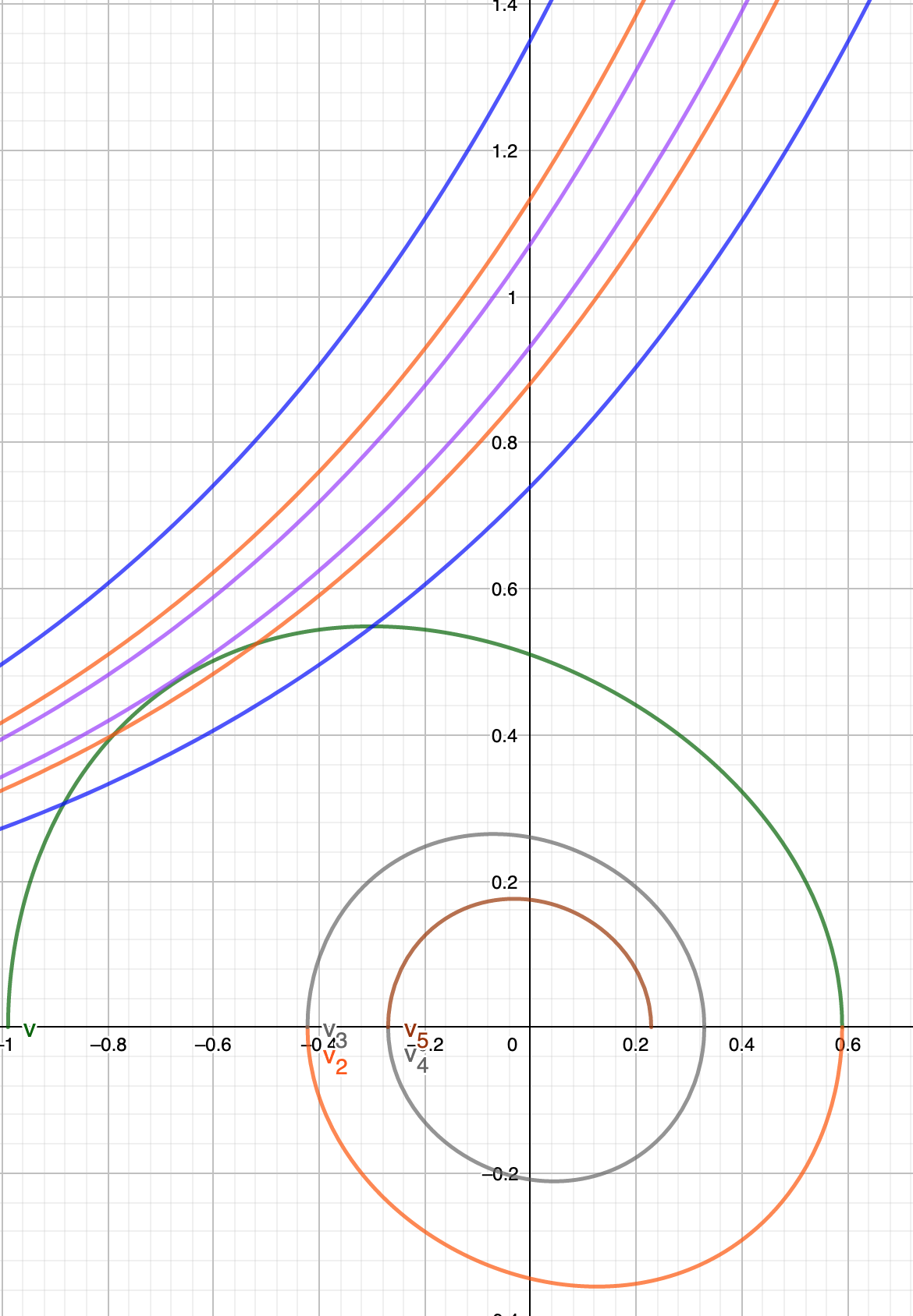
Because of how $H_n(X)$ and $L_n(X)$ cramped together, I only included the first three cycles. Exponential line above $V^2=1$ corresponds to $L_n(X)$. Exponential line below $V^2=1$ corresponds to $H_n(X)$. Each color of the line corresponds to the phase cycle plot directly below.

From what I observed in the graph. I understand that:

1. The closer $H_n(X)$ to cross $(X,V)=(0,1)$, that means the closer the cycle to the final state. Cycle with $K=0$ is defined with $H(X)=$ everywhere (the furthest from final state)
2. The closer $L_n(X)$ to cross $(X,V)=(0,1)$, that means the closer the cycle to the final state. Cycle with $K=0$ is defined have undefined normalized cycle length. (because division by zero). However we can intuitively says that if the value $L_n(X)$ is bigger in the same phase, that means it is furthest from the final state.

Recap of the definition and identities

From the phase and cycle plot, we summarized the following proposed definition and identities to understand the cycles.

Recursive relations

Standard base:

$X_0=-\infty \\ K_0=0 \\ X_1=1$

Recursive relation, starting from $n=1$

$X_n=(-1)^{n-1}(1+W(\frac{K_{n-1}}{e}) \\ K_n=(1+(-1)^{n-1} X_n)e^{(-1^{n-1}) X_n} \\ V_n=(-1)^n \sqrt{1+(-1)^{n-1} X- K_n e^{(-1^{n-1}) X}} \\ X_{peak-n}=(-1)^n\ln(K_n)$

Qualitative definition

• The span $S_n$ is the length from $X_{n,min}$ to $X_{n,max}$ in a given cycle n.
• The amplitude $A_n$ is the maximum displacement from the origin point to a point where the velocity is zero in a given cycle.
• The absolute amplitude difference $\Delta A$ is the difference between the left amplitude and right amplitude of the given cycle, relative to the origin point.

Quantitative definition

The absolute cycle length $H_n(X)$ quantifies how far the current cycle $n$ into the final cycle state $n=\infty$.

$H_n(X)=K_n e^X$

Absolute cycle length preserves ordering. Whenever $b > a$, $H_b(X) > H_a(X)$ if compared in the same value of X. Maximum value is $H_n(X)=e^X$.

Relative cycle length is a quantity to measure the ordering of the cycle $H_{ba}(X)=\frac{H_b(X)}{H_a(X)}$, if compared in the same value of X.

Cycle average is a quantity that measures the average of two cycles. $H_{avg}=\sqrt{H_a \cdot H_b}$

Hyperbolic phase angle $\phi_n(X)$ quantifies the phase of motion in the current cycle n. It can be used for ordering in the same cycle (but with some care about the parity).

$\phi_n(X)=\frac{X}{2}+\frac{1}{2}\ln(K_n)$

The mid of the half cycle phase corresponds to when the acceleration is zero.

$\phi_{n,mid}=X_{peak-n}=\ln(K_n)$

The minima and maxima of the phase in a given cycle $n$ is completely determined from the current span $S_n$ and amplitude difference $\Delta A$.

$\phi_{n,min}=-\frac{S_n+\Delta A_n}{4}+\frac{1}{2}\ln(K_n) \\ \phi_{n,max}=\frac{S_n-\Delta A_n}{4}+\frac{1}{2}\ln(K_n)$

The phase angle difference is the difference between two phases. $\Delta \phi=\phi_b-\phi_a$

The normalized phase angle $\Phi_n(X)$ is a translated phase where the origin is $\phi_{n,mid}$. The normalized phase angle has a special property that the sign can also determined the sign of the equation of motions (combination of sign of acceleration, and velocity).

$\Phi_n(X) = \phi_n(X)-\phi_{mid}=\frac{1}{2}\ln(\frac{e^X}{K_n}) \\ \Phi_{n,mid}(X)=0 \\ \Phi_{n,min}=-\frac{S+\Delta A}{4}-\frac{1}{2}\ln(K_n) \\ \Phi_{n,max}=\frac{S-\Delta A}{4}-\frac{1}{2}\ln(K_n)$

The normalized phase angle difference is the same phase angle difference, $\Delta \Phi=\Delta \phi$.

From the normalized phase angle, we can construct a normalized cycle length $L_n(X)$. The contour of $L_n(X)$ preserves ordering between cycles.

$L_n(X)=\frac{e^X}{K_n}$

Relation and identities

For any $X_a$ and $X_b$, with $b>a$, with the same squared velocity $V^2$, it follows:

$H_{avg} sinh(\Delta \phi) = \frac{\Delta X}{2} \\$

Expanded as:

$\sqrt{H_a \cdot H_b} sinh(\frac{\phi_b-\phi_a}{2}) = \frac{X_b-X_a}{2}$

Above equation assumes both odd parity cycle $n$. If one of the arguments is even cycle, switch the sign of $X$. If both $X$ is even cycle, switch both sign.

If expanded, odd b and a:

$\sqrt{K_b K_a} e^{\frac{X_b+X_a}{2}} sinh(\ln(\sqrt{\frac{K_b}{K_a}})+\frac{X_b-X_a}{2})=\frac{X_b-X_a}{2}$

odd b, even a:

$\sqrt{K_b K_a} e^{\frac{X_b-X_a}{2}} sinh(\ln(\sqrt{\frac{K_b}{K_a}})+\frac{X_b+X_a}{2})=\frac{X_b+X_a}{2}$

even b, even a:

$\sqrt{K_b K_a} e^{\frac{-X_b-X_a}{2}} sinh(\ln(\sqrt{\frac{K_b}{K_a}})+\frac{X_b-X_a}{2})=\frac{X_b-X_a}{2}$

even b, odd a:

$\sqrt{K_b K_a} e^{\frac{-X_b+X_a}{2}} sinh(\ln(\sqrt{\frac{K_b}{K_a}})+\frac{X_b+X_a}{2})=\frac{X_b+X_a}{2}$

If it is the same cycle, relation reduced to:

if odd:

$Ke^{\frac{X_b+X_a}{2}} sinh(\frac{X_b-X_a}{2})=\frac{X_b-X_a}{2}$

if even:

$Ke^{\frac{-X_b-X_a}{2}} sinh(\frac{X_b-X_a}{2})=\frac{X_b-X_a}{2}$

If both $X$ are zeroes in the same cycle, relation is simplified into:

$Ke^{\frac{\Delta A}{2}}sinh(\frac{S}{2})=\frac{S}{2}$

Some defition have connecting relation:

The relation below happens in the same cycle n:

$\Delta \Phi_n = \Delta \phi_n$

The relation below connects between $\phi_n(X)$, $H_n(X)$, $L_n(X)$ and $\Phi_n(X)$ in the same cycle n:

$\phi_n(X)=\frac{1}{2}\ln(H_n(X)) \\ \Phi_n(X)=\frac{1}{2}\ln(\frac{H_n(X)}{K_n^2})=\frac{1}{2}\ln(L_n(X)) \\ L_n(X)=\frac{H_n(X)}{K_n^2} \\ H_n(X)=e^{2\phi_n(X)} \\ L_n(X)=e^{2\Phi_n(X)}$